Dans la nouvelle version de unifiedml disponible sur CRAN, vous pouvez comparer différents modèles à l’aide de la validation croisée k-fold (section 1 de ce billet de blog), et il existe une interface unifiée pour prédire les probabilités du modèle (section 2 de ce billet de blog).
install.packages("unifiedml")

install.packages(c("e1071", "randomForest", "caret"))

install.packages("glmnet")

library(unifiedml)
set.seed(123)
X <- iris[, 1:4]
y <- iris$Species
models <- list( # `Model` is exported from package 'unifiedml'
glm = Model$new(caret::train), # caret can be used (see
rf = Model$new(randomForest::randomForest), # or a native pkg
svm = Model$new(e1071::svm) # or another pkg
)
params <- list(
glm = list(method = "glmnet",
tuneGrid = data.frame(alpha = 0, lambda = 0.01), # for caret model, all hyperparameters must be provided
trControl = trainControl(method = "none")),
rf = list(ntree = 150), # Not necessarily needing to specify all hyperparameters
svm = list(kernel = "radial",
cost = 1,
gamma = 0.1)
)
results <- unifiedml::benchmark(models, X, y, cv = 5, params = params)
[1/3] Fitting model: glm
Mean CV score for glm: 0.9533
[2/3] Fitting model: rf
Mean CV score for rf: 0.9600
[3/3] Fitting model: svm
Mean CV score for svm: 0.9733
print(results) # 5-fold cross-validation results
$glm
$glm$avg_score
[1] 0.9533333
$glm$scores
fold1 fold2 fold3 fold4 fold5
0.9333333 0.9666667 0.9333333 0.9333333 1.0000000
$rf
$rf$avg_score
[1] 0.96
$rf$scores
fold1 fold2 fold3 fold4 fold5
0.9333333 1.0000000 0.9333333 0.9333333 1.0000000
$svm
$svm$avg_score
[1] 0.9733333
$svm$scores
fold1 fold2 fold3 fold4 fold5
0.9666667 1.0000000 0.9666667 0.9333333 1.0000000
# initialize empty vectors
model_vec <- c()
fold_vec <- c()
score_vec <- c()
for (model in names(results)) {
scores <- results[[model]]$scores
model_vec <- c(model_vec, rep(model, length(scores)))
fold_vec <- c(fold_vec, names(scores))
score_vec <- c(score_vec, as.numeric(scores))
}
df <- data.frame(
model = model_vec,
fold = fold_vec,
score = score_vec
)
library(ggplot2)
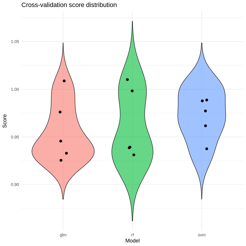
ggplot(df, aes(x = model, y = score, fill = model)) +
geom_violin(trim = FALSE, alpha = 0.6) +
geom_jitter(width = 0.08, size = 2) +
theme_minimal() +
labs(
title = "Cross-validation score distribution",
x = "Model",
y = "Score"
) +
theme(legend.position = "none")

# Load required packages
library(unifiedml)
library(randomForest)
library(nnet)
library(e1071)

# Load iris dataset
data(iris)

# Setup reproducible data
set.seed(42)

# Create feature matrix (all 4 numeric features)
X <- as.matrix(iris[, 1:4])
colnames(X) <- c("Sepal.Length", "Sepal.Width", "Petal.Length", "Petal.Width")

# Target: Species (multi-class with 3 levels)
y_multiclass <- iris$Species

# Create binary classification target (Versicolor vs others)
y_binary <- factor(
  ifelse(iris$Species == "versicolor", "versicolor", "other"),
  levels = c("other", "versicolor")
)

# Split into train/test (75% train, 25% test)
set.seed(42)
train_idx <- sample(1:nrow(X), size = floor(0.75 * nrow(X)), replace = FALSE)
test_idx <- setdiff(1:nrow(X), train_idx)

X_train <- X[train_idx, ]
X_test <- X[test_idx, ]
y_train_multiclass <- y_multiclass[train_idx]
y_test_multiclass <- y_multiclass[test_idx]
y_train_binary <- y_binary[train_idx]
y_test_binary <- y_binary[test_idx]

cat("\n")
cat("============================================================================\n")
cat("IRIS DATASET - Summary\n")
cat("============================================================================\n")
cat(sprintf("Training samples: %d\n", nrow(X_train)))
cat(sprintf("Test samples: %d\n", nrow(X_test)))
cat(sprintf("Features: %d\n", ncol(X_train)))
cat(sprintf("Classes: %s\n", paste(levels(y_multiclass), collapse = ", ")))

# ============================================================================
# EXAMPLE 1: randomForest - Multi-class Classification on IRIS
# ============================================================================

cat("\n")
cat("============================================================================\n")
cat("EXAMPLE 1: randomForest - Multi-class Classification\n")
cat("============================================================================\n")

mod_rf <- Model$new(randomForest::randomForest)
mod_rf$fit(X_train, y_train_multiclass, ntree = 100)

cat("\nPredicting probabilities for first 5 test samples:\n")
probs_rf <- mod_rf$predict_proba(X_test[1:5, ])

cat("\nProbability matrix:\n")
print(round(probs_rf, 3))

cat("\nInterpretation:\n")
for(i in 1:5) {
  cat(sprintf("\nSample %d (Actual: %s):\n", i, as.character(y_test_multiclass[i])))
  cat(sprintf("  setosa:     %.1f%%\n", probs_rf[i, "setosa"] * 100))
  cat(sprintf("  versicolor: %.1f%%\n", probs_rf[i, "versicolor"] * 100))
  cat(sprintf("  virginica:  %.1f%%\n", probs_rf[i, "virginica"] * 100))
  cat(sprintf("  Predicted:  %s\n", colnames(probs_rf)[which.max(probs_rf[i, ])]))
}

# Get class predictions
pred_classes_rf <- mod_rf$predict(X_test[1:5, ], type = "class")
cat("\nPredicted classes (first 5):", as.character(pred_classes_rf), "\n")
cat("Actual classes (first 5):   ", as.character(y_test_multiclass[1:5]), "\n")

# Calculate accuracy on full test set
probs_all_rf <- mod_rf$predict_proba(X_test)
pred_all_rf <- colnames(probs_all_rf)[apply(probs_all_rf, 1, which.max)]
accuracy_rf <- mean(pred_all_rf == as.character(y_test_multiclass))
cat(sprintf("\nTest set accuracy: %.1f%%\n", accuracy_rf * 100))

# ============================================================================
# EXAMPLE 2: nnet - Multi-class Classification on IRIS
# ============================================================================

cat("\n")
cat("============================================================================\n")
cat("EXAMPLE 2: nnet - Multi-class Classification\n")
cat("============================================================================\n")

mod_nnet <- Model$new(nnet::nnet)
mod_nnet$fit(X_train, y_train_multiclass, size = 10, maxit = 200, trace = FALSE)

cat("\nPredicting probabilities for first 5 test samples:\n")
probs_nnet <- mod_nnet$predict_proba(X_test[1:5, ])

cat("\nProbability matrix (all 3 classes):\n")
print(round(probs_nnet, 3))

cat("\nDetailed predictions:\n")
for(i in 1:5) {
  cat(sprintf("\nSample %d (Actual: %s):\n", i, as.character(y_test_multiclass[i])))
  cat(sprintf("  setosa:     %.1f%%\n", probs_nnet[i, "setosa"] * 100))
  cat(sprintf("  versicolor: %.1f%%\n", probs_nnet[i, "versicolor"] * 100))
  cat(sprintf("  virginica:  %.1f%%\n", probs_nnet[i, "virginica"] * 100))
  cat(sprintf("  Predicted:  %s\n", colnames(probs_nnet)[which.max(probs_nnet[i, ])]))
}

# Get class predictions
pred_classes_nnet <- mod_nnet$predict(X_test[1:5, ], type = "class")
cat("\nPredicted classes (first 5):", as.character(pred_classes_nnet), "\n")
cat("Actual classes (first 5):   ", as.character(y_test_multiclass[1:5]), "\n")

# Calculate accuracy
probs_all_nnet <- mod_nnet$predict_proba(X_test)
pred_all_nnet <- colnames(probs_all_nnet)[apply(probs_all_nnet, 1, which.max)]
accuracy_nnet <- mean(pred_all_nnet == as.character(y_test_multiclass))
cat(sprintf("\nTest set accuracy: %.1f%%\n", accuracy_nnet * 100))

# ============================================================================
# EXAMPLE 3: SVM - Multi-class Classification on IRIS
# ============================================================================

cat("\n")
cat("============================================================================\n")
cat("EXAMPLE 3: SVM - Multi-class Classification\n")
cat("============================================================================\n")

mod_svm <- Model$new(e1071::svm)
mod_svm$fit(X_train, y_train_multiclass, probability = TRUE, kernel = "radial")

cat("\nPredicting probabilities for first 5 test samples:\n")
probs_svm <- mod_svm$predict_proba(X_test[1:5, ])

cat("\nProbability matrix:\n")
print(round(probs_svm, 4))

cat("\nDetailed predictions:\n")
for(i in 1:5) {
  cat(sprintf("\nSample %d (Actual: %s):\n", i, as.character(y_test_multiclass[i])))
  cat(sprintf("  setosa:     %.1f%%\n", probs_svm[i, "setosa"] * 100))
  cat(sprintf("  versicolor: %.1f%%\n", probs_svm[i, "versicolor"] * 100))
  cat(sprintf("  virginica:  %.1f%%\n", probs_svm[i, "virginica"] * 100))
  cat(sprintf("  Predicted:  %s\n", colnames(probs_svm)[which.max(probs_svm[i, ])]))
}

# Calculate accuracy
probs_all_svm <- mod_svm$predict_proba(X_test)
pred_all_svm <- colnames(probs_all_svm)[apply(probs_all_svm, 1, which.max)]
accuracy_svm <- mean(pred_all_svm == as.character(y_test_multiclass))
cat(sprintf("\nTest set accuracy: %.1f%%\n", accuracy_svm * 100))

============================================================================
IRIS DATASET - Summary
============================================================================
Training samples: 112
Test samples: 38
Features: 4
Classes: setosa, versicolor, virginica

============================================================================
EXAMPLE 1: randomForest - Multi-class Classification
============================================================================

Predicting probabilities for first 5 test samples:

Probability matrix:
  setosa versicolor virginica
1      1          0         0
2      1          0         0
3      1          0         0
4      1          0         0
5      1          0         0
attr(,"assign")
[1] 1 1 1
attr(,"contrasts")
attr(,"contrasts")$pred
[1] "contr.treatment"

attr(,"extraction_method")
[1] "fallback::1"
attr(,"model_class")
[1] "randomForest.formula"

Interpretation:

Sample 1 (Actual: setosa):
  setosa:     100.0%
  versicolor: 0.0%
  virginica:  0.0%
  Predicted:  setosa

Sample 2 (Actual: setosa):
  setosa:     100.0%
  versicolor: 0.0%
  virginica:  0.0%
  Predicted:  setosa

Sample 3 (Actual: setosa):
  setosa:     100.0%
  versicolor: 0.0%
  virginica:  0.0%
  Predicted:  setosa

Sample 4 (Actual: setosa):
  setosa:     100.0%
  versicolor: 0.0%
  virginica:  0.0%
  Predicted:  setosa

Sample 5 (Actual: setosa):
  setosa:     100.0%
  versicolor: 0.0%
  virginica:  0.0%
  Predicted:  setosa

Predicted classes (first 5): setosa setosa setosa setosa setosa
Actual classes (first 5):    setosa setosa setosa setosa setosa

Test set accuracy: 94.7%

============================================================================
EXAMPLE 2: nnet - Multi-class Classification
============================================================================

Predicting probabilities for first 5 test samples:

Probability matrix (all 3 classes):
  setosa versicolor virginica
1      1          0         0
2      1          0         0
3      1          0         0
4      1          0         0
5      1          0         0
attr(,"extraction_method")
[1] "fallback::5"
attr(,"model_class")
[1] "nnet.formula"

Detailed predictions:

Sample 1 (Actual: setosa):
  setosa:     100.0%
  versicolor: 0.0%
  virginica:  0.0%
  Predicted:  setosa

Sample 2 (Actual: setosa):
  setosa:     100.0%
  versicolor: 0.0%
  virginica:  0.0%
  Predicted:  setosa

Sample 3 (Actual: setosa):
  setosa:     100.0%
  versicolor: 0.0%
  virginica:  0.0%
  Predicted:  setosa

Sample 4 (Actual: setosa):
  setosa:     100.0%
  versicolor: 0.0%
  virginica:  0.0%
  Predicted:  setosa

Sample 5 (Actual: setosa):
  setosa:     100.0%
  versicolor: 0.0%
  virginica:  0.0%
  Predicted:  setosa

Predicted classes (first 5): setosa setosa setosa setosa setosa
Actual classes (first 5):    setosa setosa setosa setosa setosa

Test set accuracy: 97.4%

============================================================================
EXAMPLE 3: SVM - Multi-class Classification
============================================================================

Predicting probabilities for first 5 test samples:

Probability matrix:
  setosa versicolor virginica
1      1          0         0
2      1          0         0
3      1          0         0
4      1          0         0
5      1          0         0
attr(,"assign")
[1] 1 1 1
attr(,"contrasts")
attr(,"contrasts")$pred
[1] "contr.treatment"

attr(,"extraction_method")
[1] "fallback::1"
attr(,"model_class")
[1] "svm.formula"

Detailed predictions:

Sample 1 (Actual: setosa):
  setosa:     100.0%
  versicolor: 0.0%
  virginica:  0.0%
  Predicted:  setosa

Sample 2 (Actual: setosa):
  setosa:     100.0%
  versicolor: 0.0%
  virginica:  0.0%
  Predicted:  setosa

Sample 3 (Actual: setosa):
  setosa:     100.0%
  versicolor: 0.0%
  virginica:  0.0%
  Predicted:  setosa

Sample 4 (Actual: setosa):
  setosa:     100.0%
  versicolor: 0.0%
  virginica:  0.0%
  Predicted:  setosa

Sample 5 (Actual: setosa):
  setosa:     100.0%
  versicolor: 0.0%
  virginica:  0.0%
  Predicted:  setosa

Test set accuracy: 94.7%
En rapport
PakarPBN
A Private Blog Network (PBN) is a collection of websites that are controlled by a single individual or organization and used primarily to build backlinks to a “money site” in order to influence its ranking in search engines such as Google. The core idea behind a PBN is based on the importance of backlinks in Google’s ranking algorithm. Since Google views backlinks as signals of authority and trust, some website owners attempt to artificially create these signals through a controlled network of sites.
In a typical PBN setup, the owner acquires expired or aged domains that already have existing authority, backlinks, and history. These domains are rebuilt with new content and hosted separately, often using different IP addresses, hosting providers, themes, and ownership details to make them appear unrelated. Within the content published on these sites, links are strategically placed that point to the main website the owner wants to rank higher. By doing this, the owner attempts to pass link equity (also known as “link juice”) from the PBN sites to the target website.
The purpose of a PBN is to give the impression that the target website is naturally earning links from multiple independent sources. If done effectively, this can temporarily improve keyword rankings, increase organic visibility, and drive more traffic from search results.
